Generative Model Landscape

Why You Need This Mental Model

Imagine you have a photograph. You add a tiny bit of static noise — like bad TV reception. Add more. And more. Eventually, the image is pure random noise. No trace of the original. Now imagine training a neural network that can look at a noisy image and predict: "Here's what a slightly less noisy version looks like." That is diffusion. The entire idea.

But diffusion is not the only approach. Four families of generative models compete in the image generation space, and understanding their tradeoffs helps you make informed engineering decisions about which services and models to use.

The Four Generative Model Families

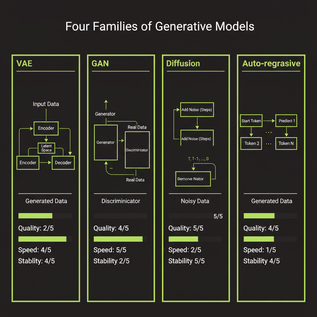
VAE (Variational Autoencoders)

The idea: compress an image into a small "latent" vector, then decompress it back. Train the model so the latent space is smooth and continuous — nearby points produce similar images.

Image → [Encoder] → Latent vector (z) → [Decoder] → Reconstructed image

Strengths: Fast generation (single forward pass through the decoder), smooth and interpretable latent space where you can interpolate between images, and stable training. Weaknesses: Outputs tend to be blurry — the model averages over possibilities instead of committing to sharp details.

VAEs are not used alone for generation anymore, but they play a critical role inside modern systems. Stable Diffusion uses a VAE to compress images before applying diffusion in the latent space. You will encounter this architecture later in this module.

GAN (Generative Adversarial Networks)

Two networks compete. A generator creates fake images. A discriminator tries to distinguish real from fake. They push each other to improve:

Random noise → [Generator] → Fake image
                                     ↓
Real image → [Discriminator] → "Real or fake?"

Strengths: Sharp, detailed outputs (the discriminator forces crisp details) and fast generation. GANs dominated image generation from ~2014–2021 — StyleGAN produced those uncanny realistic faces. Weaknesses: Training is unstable (the generator and discriminator can oscillate, collapse, or diverge), mode collapse (the generator learns to produce only a few types of images), and no natural way to condition on text prompts.

Diffusion Models: the current champion

Start with a clean image, gradually add noise until it is pure static. Then train a neural network to reverse the process — to denoise step by step:

FORWARD PROCESS (destroying information):
Photo → slightly noisy → noisier → ... → pure noise

REVERSE PROCESS (creating information):
Pure noise → slightly cleaner → cleaner → ... → new photo

Strengths: Best image quality of any approach — sharp, diverse, and coherent. Stable training with no adversarial dynamics. Easy to condition on text, other images, or sketches. Diverse outputs without mode collapse. Weaknesses: Slow generation (requires 20–50 denoising steps), computationally expensive per image, and higher latency than GANs or VAEs.

Auto-regressive (for images)

Treat an image as a sequence of tokens (like text) and predict each one in order. Quantize image patches into a vocabulary, then use a transformer to predict the next patch:

[patch_1] → predict → [patch_2] → predict → [patch_3] → ...

Strengths: Unified architecture with text (same transformer approach), naturally handles text-and-image sequences together, and scales with compute like language models. Weaknesses: Very slow (must generate one patch at a time, sequentially) and image quality historically lagged behind diffusion. However, some frontier models (GPT-4o's image generation) use auto-regressive approaches, suggesting this family may close the gap as scale increases.

Why diffusion won (for now)

Model           | Quality  | Speed    | Stability
----------------|----------|----------|-----------
VAE             | Low      | Fast     | High
GAN             | High     | Fast     | Low
Diffusion       | Highest  | Slow     | High
Auto-regressive | Good     | Slowest  | High

Diffusion models hit the sweet spot: they match or exceed GAN quality without the training headaches. The speed problem is being actively addressed — techniques like latent diffusion, distillation, and rectified flow have brought generation from hundreds of steps down to 1–4 steps.

The Diffusion Pipeline — Step by Step

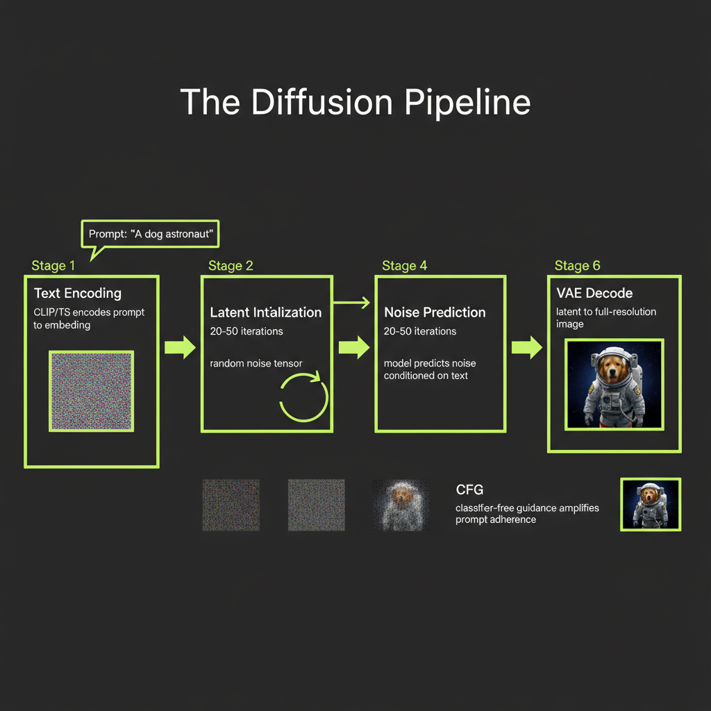
When you send a prompt to an image generation API, here is what happens on the server:

Step 1 — Text encoding

Your text prompt goes through a text encoder (CLIP or T5) to produce an embedding vector. CLIP was trained to align text and image embeddings in the same space — it understands visual concepts well but is limited to 77 tokens. T5 is a general-purpose text encoder that handles long, detailed prompts and compositional understanding better. Modern models like Stable Diffusion 3 and Flux use both encoders — CLIP for visual-semantic alignment plus T5 for rich language understanding.

Step 2 — Latent initialization

A random noise tensor is generated (or seeded for reproducibility). Instead of working with full-resolution images (512x512x3 = 786,432 values), latent diffusion compresses images using a pre-trained VAE to a 64x64 latent space — 64x smaller. This is the key innovation behind Stable Diffusion: diffuse in compressed space for the same quality at dramatically faster speed.

Step 3 — Denoising loop

The diffusion model runs 20–50 denoising steps in the compressed latent space. At each step, it looks at the noisy latent and predicts what a slightly less noisy version looks like. The model does not predict the clean image directly — it predicts the noise, and that noise is subtracted to produce a cleaner version.

Step 4 — Noise prediction conditioned on text

At every denoising step, the text embedding is injected into the model via cross-attention. This steers the denoising process: instead of denoising toward "any plausible image," the model denoises toward "a plausible image that matches this text description."

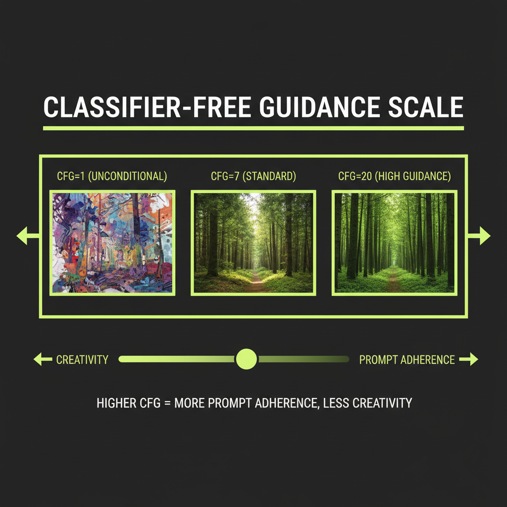
Step 5 — Classifier-free guidance (CFG)

CFG controls how strongly the model follows the text prompt. At each step, the model runs twice: once with the text prompt (conditional) and once without (unconditional). The difference is amplified by a guidance_scale parameter:

final = unconditional + guidance_scale * (conditional - unconditional)

guidance_scale = 1.0   → barely follows prompt (creative, incoherent)
guidance_scale = 7.5   → standard (good balance)
guidance_scale = 15+   → very literal (sharp but can look artificial)

This is the same concept as "temperature" for text generation — a dial between creativity and adherence. Most APIs expose this as guidance_scale or cfg_scale.

Step 6 — VAE decode

After all denoising steps, the clean latent is converted back to a full-resolution pixel image by the VAE decoder. Total GPU time: 2–10 seconds depending on model and resolution.

Architecture Evolution

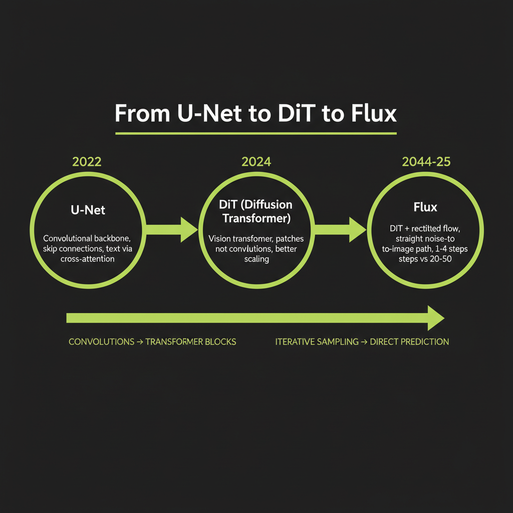
U-Net (Stable Diffusion 1.x/2.x)

The first wave of latent diffusion models used a U-Net — a convolutional neural network shaped like the letter U. The downsampling path compresses the noisy latent to capture global structure. The bottleneck processes with attention layers (where text conditioning happens via cross-attention). The upsampling path reconstructs details at full resolution. Skip connections pass fine details directly between the two paths.

U-Nets worked well but hit scaling limits. You can make a U-Net bigger, but improvements plateau — the same pattern that happened when RNNs were replaced by transformers in NLP.

DiT — Diffusion Transformers (DALL-E 3, Stable Diffusion 3)

In 2023, the DiT paper showed that you could replace the U-Net with a plain vision transformer — and it scaled much better. The key changes: split the latent into patches and treat them as a sequence (like ViT does for classification), use standard transformer blocks with self-attention and feed-forward layers, and inject the timestep via adaptive layer normalization.

DiT gave diffusion models the same scaling properties that made GPT-4 possible. More parameters, more data, more compute = better results. The same architectural insight that transformed NLP works just as well for images.

Flux: DiT + Rectified Flow (current SOTA)

Flux (from Black Forest Labs, the team behind Stable Diffusion) combines DiT with rectified flow. Standard diffusion adds noise in a curved path — the reverse process follows a curved trajectory through latent space. Rectified flow straightens this path into a nearly straight line:

Standard diffusion path:     Rectified flow path:
noise ~~~>                   noise
          ~~~>                   \
               ~~~> image         \→ image

A straight path can be traversed in fewer steps. Standard diffusion needs 20–50 steps. Rectified flow models produce good results in 1–4 steps — a 5–50x speedup. The Flux model family includes Flux.1 [schnell] (fastest, 1–4 steps, ~$0.003/image), Flux.1 [dev] (open-weight, good quality), and Flux.1 [pro] (best quality, API-only).

Text-to-Video: Where the Field Is Going

Text-to-video extends image diffusion to the temporal dimension. Instead of denoising a single latent, denoise a sequence of latents with temporal consistency.

• Sora (OpenAI): Uses "spacetime patches" — treats video frames as a 3D grid of patches processed by a DiT. Can generate variable lengths and resolutions.
• Runway Gen-3 Alpha: Production-available through API. Focus on controllability — camera motion, style transfer, image-to-video.
• Kling (Kuaishou): Strong results from China's short-video ecosystem. Good at human motion and complex scenes.

What This Means for Engineering Decisions

Choosing between models

• Flux schnell (~$0.003/image, ~1 second): Development and prototyping. Never prototype with expensive models.
• Flux dev (~$0.025/image, ~5 seconds): Production quality at reasonable cost.
• DALL-E 3: When you need OpenAI's content policy filtering or illustration style.

CFG scale as a tuning lever

Higher guidance scale = more prompt adherence but potentially artificial-looking results. Lower guidance scale = more creative interpretation but less control. Start at 7.5 and adjust based on your use case.

Steps vs quality

With rectified flow models like Flux schnell, 1–4 steps is sufficient. With standard diffusion models, 20–30 steps is the practical range. More steps means more GPU time and higher cost per image.