How Transformers Work
Trace data through the architecture you use every day — from raw text to predicted token.
What you'll learn
Why You Need This Mental Model
You already call Claude's API every day. This module explains what happens between your prompt and the response — and why that knowledge makes you a better engineer.
The gap between "I call an API" and "I understand what's happening"
Most developers treat LLMs as black boxes. You send a string, you get a string back. That works until it does not — until the model hallucinates, until your costs spike, until you cannot figure out why your 200K-token context window produces worse results than a carefully trimmed 4K prompt.
The transformer architecture is not academic trivia. It is the operating manual for every decision you will make as an AI engineer: how to structure prompts, why retrieval beats stuffing, when to use a smaller model, and what "hallucination" actually means at the mechanism level.
What this knowledge unlocks
- Better prompts: When you understand that attention is context-dependent, you know to put critical information where the model will attend to it.
- Better debugging: When a model hallucinates, you can reason about whether the feed-forward network's learned knowledge is overriding the context you provided.
- Better cost intuition: When you understand tokenization, you can estimate costs before you run a single API call.
Step 1 — Tokenization
LLMs don't see text — they see integers
A transformer does not process characters, words, or sentences. It processes tokens — subword units represented as integers. Before your prompt reaches any neural network layer, it passes through a tokenizer that converts text into a sequence of token IDs.
Input text:  "Hello, world!"
Tokens:      ["Hello", ",", " world", "!"]
Token IDs:   [9906, 11, 1917, 0]
Each token ID maps to an entry in the model's fixed vocabulary — typically 32,000 to 100,000 entries for modern LLMs.
How Byte Pair Encoding (BPE) builds a vocabulary
The dominant tokenization algorithm is Byte Pair Encoding. It starts with individual characters and iteratively merges the most frequent adjacent pairs until the vocabulary reaches a target size:
Training data: "low lower lowest"

Step 0: vocabulary = {l, o, w, e, r, s, t, ' '}
Step 1: most frequent pair ('l','o') -> merge to 'lo'
Step 2: most frequent pair ('lo','w') -> merge to 'low'
Step 3: most frequent pair ('e','r') -> merge to 'er'
Step 4: most frequent pair ('low','er') -> merge to 'lower'
...
After training, common words like "the" become single tokens. Rare words like "defenestration" might be split into ["def", "en", "est", "ration"].
The rule of thumb: ~1 token = 4 characters
In English prose, 1 token is approximately 4 characters or 0.75 words. This ratio shifts significantly for other content types:
"Hello world"           -> 2 tokens   (English, common words)
"Antidisestablishment"  -> 4 tokens   (long, uncommon word)
"function getData()"    -> 5 tokens   (code is token-expensive)
"こんにちは"             -> 3 tokens   (non-English, less efficient)
Why non-English text and code tokenize differently
BPE vocabularies are trained on the distribution of the training data. English text dominates most training corpora, so English words get efficient single-token representations. Code, mathematical notation, and non-Latin scripts are underrepresented, so they require more tokens per semantic unit. This directly affects cost — a Japanese prompt costs more tokens than its English equivalent carrying the same meaning.
Tokenization affects cost. A verbose prompt is an expensive prompt. When you understand that every token has a price, you start writing prompts that are precise rather than padded. This intuition becomes critical when you are making thousands of API calls per day in production.
Step 2 — Token Embeddings
Mapping token IDs to high-dimensional vectors
Each token ID is mapped to an embedding vector — a point in high-dimensional space. For Claude, these vectors have thousands of dimensions (frontier models typically use 4,096 to 12,288 dimensions). The embedding layer is a lookup table: token ID 9906 maps to a specific vector of floating-point numbers.
What embedding space captures: semantic proximity
The key property of embedding space is that semantically similar tokens are nearby. The vectors for "king" and "queen" are closer together than "king" and "refrigerator." This geometric relationship is what allows the model to generalize — it can apply what it learned about one concept to similar concepts, because they occupy neighboring regions in the space.
Positional encoding — RoPE for modern models
Transformers process all tokens in parallel, not sequentially like RNNs. But word order matters — "dog bites man" is not the same as "man bites dog." Positional encoding adds position information to each embedding so the model knows where each token sits in the sequence.
Modern models like Claude use RoPE (Rotary Position Embeddings): position is encoded as a rotation in the embedding space. This is why models have context length limits — the rotation patterns are trained up to a certain position. Going beyond that trained limit degrades performance because the model encounters position encodings it has never seen.
Step 3 — Self-Attention
Query, Key, Value vectors — the lookup mechanism
Self-attention is the core mechanism that makes transformers powerful. For each token, the model computes three vectors by multiplying the token's embedding by three learned weight matrices:
- Query (Q): "What am I looking for?" — what information this token needs from other tokens.
- Key (K): "What do I contain?" — what information this token advertises to others.
- Value (V): "What information do I provide?" — the actual content that gets mixed in.
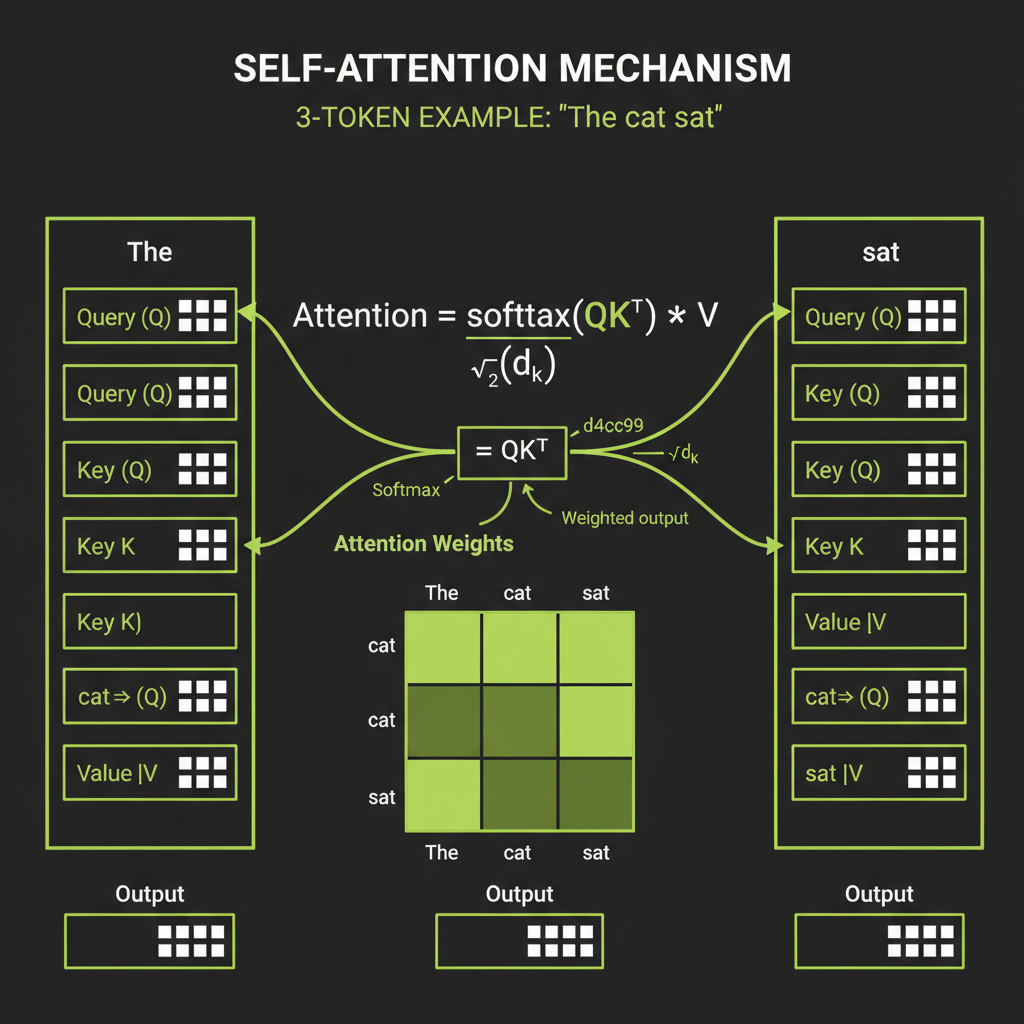
Attention weights: softmax(QKT / sqrt(d)) * V
The attention computation is a scaled dot-product:
Attention(Q, K, V) = softmax(Q * K^T / sqrt(d)) * VHere is the intuition: Q and K determine the attention weights — which tokens are relevant to each other. The dot product of Q and K produces a score; higher scores mean stronger relevance. The sqrt(d) scaling prevents the dot products from growing too large in high-dimensional space (which would push softmax into regions where gradients vanish). The resulting weights are applied to V to produce the output — a weighted mix of information from all relevant tokens.
What attention learns
Consider the sentence "The cat sat on the mat." When processing the token "sat," the attention mechanism might heavily attend to "cat" (who is sitting?) and "mat" (where?). The attention weights form a matrix showing these relationships — and the model learns these patterns during training.
Multi-head attention: parallel perspectives
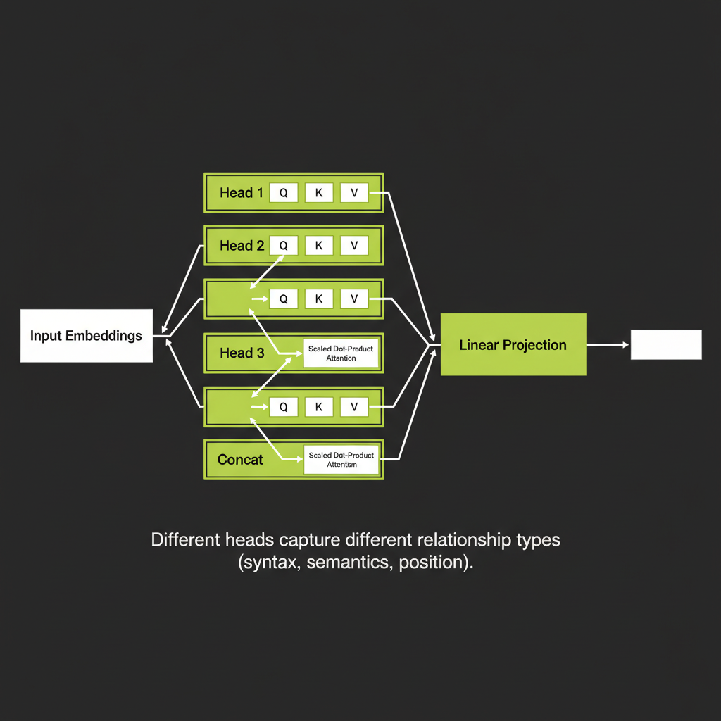
Instead of computing one attention pattern, the model runs multiple attention heads in parallel (32 to 128 heads in frontier models). Each head can learn a different type of relationship:
- Head 1 might learn subject-verb relationships
- Head 2 might learn adjective-noun relationships
- Head 3 might learn positional or structural patterns
- Head 4 might learn coreference (pronouns to nouns)
After all heads compute independently, their outputs are concatenated and projected through a linear layer to produce the combined output. This is why multi-head attention is more expressive than single-head — it can simultaneously represent many different kinds of token relationships.
Step 4 — Feed-Forward Network
Two linear projections with GELU activation
After attention, each token passes independently through a feed-forward network (FFN):
FFN(x) = GELU(x * W1 + b1) * W2 + b2This is a two-layer neural network applied to each token position separately. The FFN is where the model stores factual knowledge — associations learned during pre-training. The parameter count of the FFN layers dominates the total model size.
Why researchers call FFN layers "knowledge stores"
Attention determines which tokens are relevant to each other — it is the routing mechanism. The FFN transforms what the model knows about those tokens — it is the knowledge store. This division of labor is what makes the transformer architecture so effective: attention handles context, FFN handles knowledge.
"Hallucination as FFN overriding context" is a simplified model that provides useful intuition but is not the full picture. The actual mechanisms behind hallucination are an active area of research. This framing is pedagogically useful but should not be treated as settled fact.
"Early layers capture syntax, later layers capture semantics" is a pattern observed in interpretability research, but it is a simplification. The reality is more nuanced — representations develop gradually and different types of information are distributed across layers. Treat this as a useful mental model, not settled fact.
Step 5 — Stacking Layers and Producing Output
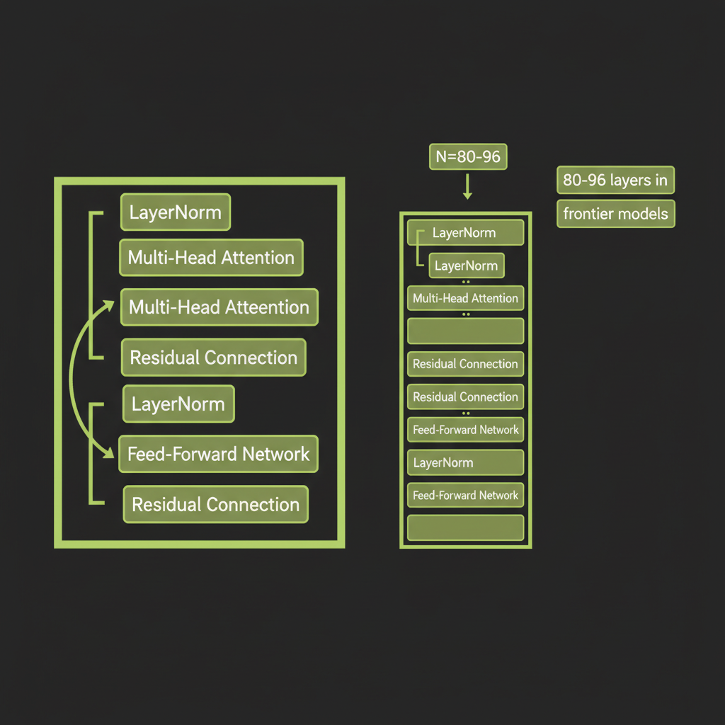
Layer normalization and residual connections
Each transformer block has two sub-layers (attention and FFN), and each is wrapped in:
- Layer normalization (modern models use RMSNorm, which is simpler and faster) — stabilizes training by normalizing the activations.
- Residual connections — the input to each sub-layer is added back to its output. This lets gradients flow directly through the network, preventing the vanishing gradient problem in deep networks.
Stacking 80–96 transformer blocks in frontier models
A complete model stacks many identical transformer blocks. Each layer refines the representation:
GPT-3:        96 layers, 96 attention heads, 12,288-dim embeddings
Llama 3 70B:  80 layers, 64 heads, 8,192-dim embeddings
Claude:       Architecture details not public, but same transformer family
Output logits to probability distribution
After the final transformer block, the model produces a logit for every token in the vocabulary — roughly 100,000 numbers. These logits are converted to probabilities using the softmax function:
Token       | Logit  | Probability
"mat"       | 3.2    | 0.23
"floor"     | 2.9    | 0.18
"couch"     | 2.5    | 0.12
"table"     | 2.1    | 0.08
"roof"      | 1.8    | 0.06
... (99,995 more tokens with smaller probabilities)
Sampling: how the next token is chosen
The model does not always pick the most probable token. Generation parameters like temperature, top-k, and top-p control how the next token is sampled from this distribution. We cover these in detail in Module 2. For now, the key insight is: the transformer produces a probability distribution, and a sampling strategy selects from it.
What This Means for You as an Engineer
Why context window size matters (attention is O(n2))
Self-attention computes a score between every pair of tokens. For a sequence of n tokens, that is n * n comparisons. Doubling your context window quadruples the attention computation. This is why 200K-token context windows are expensive — and why retrieval (finding the right 4K tokens to include) often outperforms stuffing the entire knowledge base into the prompt.
Why model quality varies by language and domain
The model's knowledge is a function of its training data distribution. English dominates most training corpora, so English performance is strongest. Code, scientific notation, and non-Latin scripts are represented but less densely. This matters for production systems — a model that excels at English customer support may underperform on Japanese legal documents, not because of architectural limits, but because of training data distribution.
The engineering implication of knowing the architecture
Understanding the transformer gives you a decision framework for every engineering choice in this course:
- Prompt design: Structure prompts so attention can route information effectively. Put critical context near where it will be used.
- RAG vs. stuffing: Retrieval beats context-stuffing because focused context produces better attention patterns than diluted context.
- Model selection: Larger models (more layers, more heads) have more capacity but higher cost. Match model size to task complexity.
- Debugging: When output quality degrades, reason about whether the issue is attention (wrong context) or FFN (wrong knowledge).
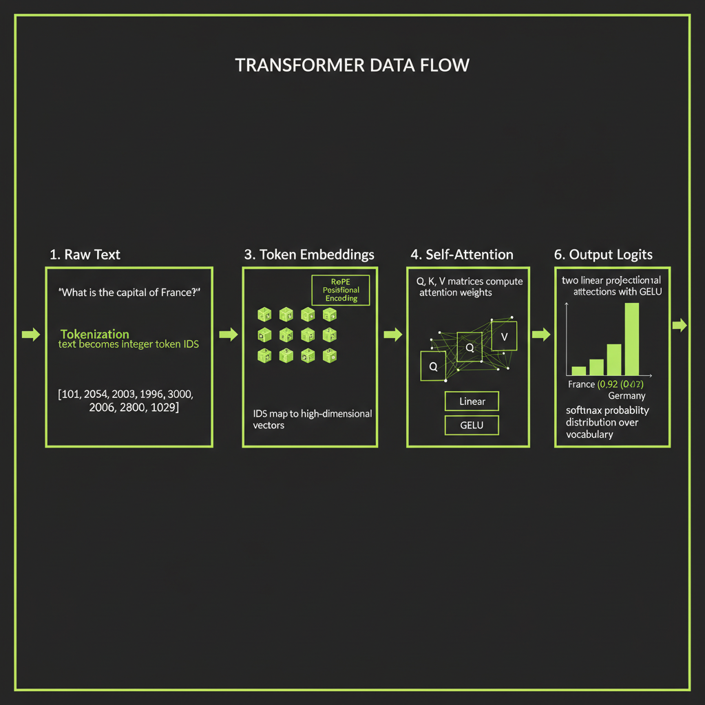
Draw or annotate a diagram tracing a single sentence through all five stages of the transformer. This exercise builds the mental model you will use throughout the course.
- Choose a short sentence — for example, "What is the capital of France?"
- Stage 1 — Tokenization: Break the sentence into tokens. Estimate how many tokens it produces (use the ~4 characters per token rule of thumb).
- Stage 2 — Embedding: Label this stage as "Token IDs mapped to 4096-dim vectors." Note that positional encoding is added here.
- Stage 3 — Attention: For each token, draw arrows to the tokens it would most likely attend to. Which word would "capital" attend to most strongly?
- Stage 4 — FFN: Label this as "Knowledge retrieval — model applies stored facts about France."
- Stage 5 — Output: Write the top 3 most probable next tokens with made-up probabilities (e.g., "Paris" 0.85, "Lyon" 0.03, "The" 0.02).
- Compare your diagram with the reference diagram at the top of this module. Note any stages you missed or misunderstood.